sx R package provides scalable spatial operations on vector and raster data using Apache SedonaDB (DataFusion-based query engine) as backend via {sedonaddb} (repo) R package. It enables efficient processing of large spatial datasets faster than with traditional R spatial packages and by utilising multi-core parallelism and out-of-memory computation. SedonaDB Rust engine and {sedonadb} R package are both in active development, so sx is currently also in an experimental stage and may change any time, especially as new features are added to the backend. Currently sx supports a subset of common spatial operations, with more planned for future releases, and it also uses DuckDB Spatial Extension for reading/writing spatial data formats that are not supported by SedonaDB native readers/writers (currently only parquet files are supported), and transfers the data to SedonaDB via Zero-Copy (or as close to it as possible). True some true larger then memory operations might not be possible just yet, as there seems to be no disk spilling support in SedonaDB just now (but it is coming!).
Implemented Functions
sx is in an experimental stage. The API may change at any time as new features are added and existing ones are improved. Use with caution and report any issues on the GitHub Issues page.
The following functions are currently implemented in sx:
Data I/O & Management
-
sx_read(),sx_write(): Read and write spatial data into/from SedonaDB backend (using SedonaDB native parquet reader/writer, but falling back to DuckDB Spatial extension for GDAL-supported formats, which is significantly faster than going throughsf::st_read/sf::st_write). -
sx_collect(): Collect results from SedonaDB into R (sf/tibble). -
sx_as_view(): Register an Rsfobject as a SedonaDB view. -
sx_create_table(): Materialize a view into a memory table. -
sx_drop_view(): Drop a registered view or table. -
sx_list(): List registered tables and views. -
sx_layers(),sx_drivers(): Inspect layers in spatial data sources and check available GDAL drivers (currently via DuckDB Spatial extension). -
sx_duckdb_to_sedona(): Use Arrow Zero-Copy to convert DuckDB tables (with spatial data) to SedonaDB views. -
sx_sql(): Execute SQL with R object interpolation.
Geometric Operations
-
sx_buffer(): Compute spatial buffers. -
sx_centroid(): Compute centroids. -
sx_envelope(): Compute bounding boxes. -
sx_simplify(): Simplify geometries. -
sx_transform(): Transform coordinate reference system. -
sx_crs(): Handle Coordinate Reference Systems. -
sx_geometry_column(): Get the name of the geometry column. -
sx_use_s2(): Control S2 geometry usage (not really fully implemented yet, more of a placeholder for future functionality).
Spatial Analysis
-
sx_join(): Perform spatial joins. -
sx_filter(): Filter data using spatial predicates. -
sx_interpolate_aw(): Areal-weighted interpolation.
Data Manipulation (dplyr)
sx supports a subset of dplyr verbs for manipulating sedonadb_dataframe objects (lazy views):
-
select(),rename(): Select and rename columns. -
mutate(): Add or modify columns (supports many Scalar functions). -
filter(): Filter rows based on conditions. -
arrange(): Sort rows. -
distinct(): Keep unique rows. -
pull(): Extract a single column as a vector. -
left_join(),inner_join(): Perform equivalent SQL joins. -
collect(): Retrieve data into R.
Configuration & Utilities
-
sx_options(): View or set package options such as message verbosity, memory and threads limits for SedonaDB and DuckDB connections (for DuckDB settings are enforced by default for connections that are created by sx (mostly for reading/writing data to/from disk), but can optionally apply to any external connections the user wants to use). -
sx_limit_duckdb_conn(): Apply memory and thread limits to any DuckDB connection. -
sx_sitrep(): System situation report.
Installation
You can install the development version of sx from GitHub with:
install.packages(
  'sedonadb',
  repos = c('https://apache.r-universe.dev', 'https://cloud.r-project.org')
)
# install.packages("pak") # if you don't have pak installed
pak::pak("e-kotov/sx")
Or from R-Universe:
install.packages('sx', repos = c('https://e-kotov.r-universe.dev', 'https://apache.r-universe.dev', 'https://cloud.r-project.org'))Example
This is a basic example showing how to perform areal-weighted interpolation using sx, mirroring the common sf workflow but backed by SedonaDB.
library(sx)
library(sf)
library(dplyr)
# 1. Load data and transform to a projected CRS (EPSG:5070)
nc <- sx_read(system.file("shape/nc.shp", package = "sf"), quiet = TRUE)
sx_crs(nc)$epsg
nc_5070 <- sx_transform(nc, 5070)
sx_crs(nc_5070)$epsg
nc_5070 <- nc_5070 |> mutate(sid = row_number())
sx_crs(nc_5070)$epsg
# 2. Create a target grid with target IDs
grid <- nc_5070 |>
st_as_sf() |>
# no st_make_grid in SedonaDB yet, so use sf
st_make_grid(n = c(10, 5)) |>
st_sf() |>
sx_as_view() |>
mutate(tid = row_number())
sx_crs(grid)$epsg
# -------------------------------------------------------------------
# Areal-Weighted Interpolation with sx
# -------------------------------------------------------------------
# (A) Extensive Interpolation (Mass-Preserving, e.g., counts)
# We treat "BIR74" as an extensive variable (count).
# weight = "total" is used here to match sf::st_interpolate_aw(extensive=TRUE) behavior,
# where the value is distributed based on the fraction of the source feature's *total area*.
# (The default weight="sum" would normalize by the sum of overlaps, which handles coverage gaps differently).
result_ext <- sx_interpolate_aw(
target = grid,
source = nc_5070,
tid = "tid",
sid = "sid",
extensive = "BIR74",
weight = "total"
)
# Check mass preservation (should be approx 1.0)
print(sum(result_ext$BIR74, na.rm = TRUE) / sum(nc$BIR74, na.rm = TRUE))
# (B) Intensive Interpolation (Spatially Intensive, e.g., rates)
# We treat "BIR74" as an intensive variable (just for demonstration purposes).
# This is equivalent to sf::st_interpolate_aw(extensive=FALSE).
# Values are averaged using the intersection area as weights.
result_int <- sx_interpolate_aw(
target = grid,
source = nc_5070,
tid = "tid",
sid = "sid",
intensive = "BIR74"
)
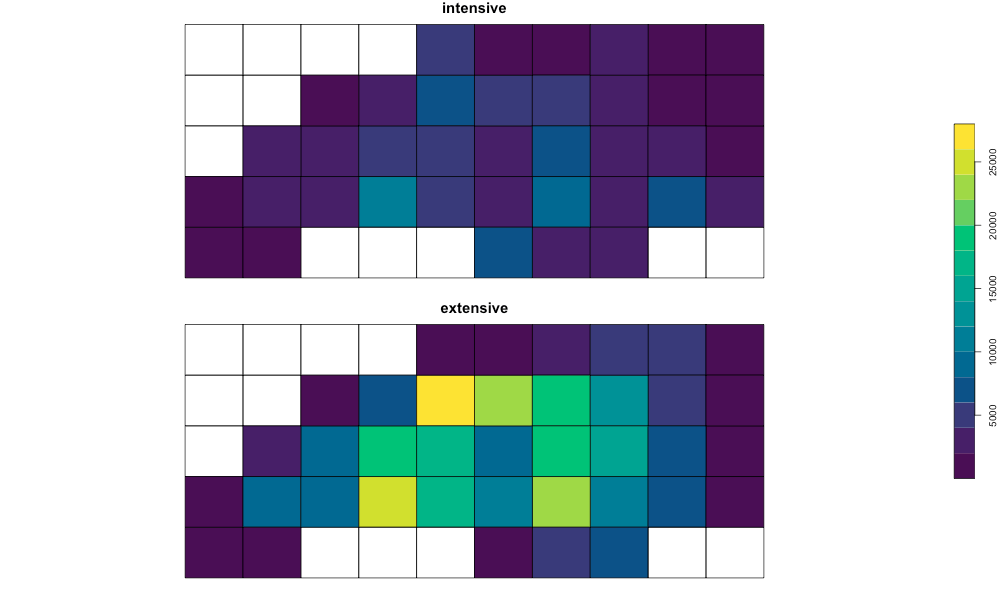
# Compare Visualization
# Combining results to plot side-by-side
results_compare <- result_ext |>
rename(
extensive = BIR74
) |>
left_join(
result_int |> select(tid, intensive = BIR74),
by = "tid"
)
# pull sf for plotting
results_compare_sf <- results_compare |> st_as_sf()
plot(
results_compare_sf[c("intensive", "extensive")],
key.pos = 4,
main = "Intensive vs Extensive Demo",
cex.main = 1.5,
pal = function(n) grDevices::hcl.colors(n, "viridis")
)
For Contributing and Development Setup see .github/CONTRIBUTING.md.