Areal-Weighted Interpolation using SedonaDB

Transfers attribute data from a source spatial layer to a target spatial layer based on the area of overlap between their geometries. All calculations are performed in SedonaDB for efficiency. Supports lazy evaluation returning sedonadb_dataframe objects.

Usage

sx_interpolate_aw(
  target,
  source,
  tid,
  sid,
  extensive = NULL,
  intensive = NULL,
  weight = "sum",
  output = NULL,
  view_name = NULL,
  keep_NA = TRUE,
  na.rm = FALSE,
  join_crs = NULL,
  verbosity = NULL,
  use_s2 = NULL,
  ...
)

Arguments

target

A sedonadb_dataframe, sf object, or view name (character) in SedonaDB representing destination geometries.

source

A sedonadb_dataframe, sf object, or view name (character) in SedonaDB containing data to interpolate.

tid

Character. Unique ID column name in target.

sid

Character. Unique ID column name in source.

extensive

Character vector. Columns in source to be treated as extensive (counts).

intensive

Character vector. Columns in source to be treated as intensive (rates).

weight

Character. Denominator for extensive variables: "sum" (default) or "total".

output

Character or NULL. Output type: sedonadb_dataframe (default), sf, tibble, geoarrow, or raw. If NULL, uses getOption("sx.output_type", "sedonadb_dataframe").

Output types:

sedonadb_dataframe: Lazy data frame (no collection).
sf: Materialized sf object.
tibble: Tibble without geometry.
geoarrow: Tibble with geoarrow_vctr geometry (Arrow-native).
raw: Tibble with geometry as raw WKB bytes (for database import).

view_name

Character (optional). Name to register the result as a persistent view in the active backend. If NULL (default), returns the result directly without creating a view.

Not all backends support named views. Check backend-specific documentation for availability.

keep_NA

Logical. If TRUE, output includes all target features (LEFT JOIN).

na.rm

Logical. If TRUE, source features with NA values are ignored.

join_crs

Numeric or Character (optional). EPSG code or WKT for CRS transform during calc.

verbosity

Character or NULL. Controls message output for this function call.

"quiet": Suppress all informational messages.
"info": Show standard progress and status messages.
"debug": Show additional diagnostic messages for troubleshooting.

If NULL (the default), uses the global sx.verbosity option. See sx_options() for persistent configuration.

use_s2

Logical or NULL. Controls spherical geometry (S2) for this operation.

TRUE: Use S2 spherical geometry (accurate for geographic coordinates).
FALSE: Use planar geometry (faster, appropriate for projected CRS).
NULL (default): Uses the global sx_use_s2() setting.

...

Ignored. Used to catch and warn about unsupported sf arguments.

Value

An sf object, sedonadb_dataframe, or tibble.

Details

Areal-weighted interpolation assumes uniform distribution of values within source polygons.

Coordinate Systems: Area calculations are sensitive to CRS. It is strongly recommended to use a projected CRS. Use the join_crs argument to project data on-the-fly during the interpolation.

Extensive vs. Intensive Variables:

Extensive (counts, sums): Value is divided proportionally to area. Use weight="sum" (relative to target coverage) or weight="total" (relative to source area).
Intensive (rates, densities): Value is averaged based on partial areas. Always uses intersection area weighting.

Examples

# \donttest{
library(sf)

# 1. Prepare Data
# Load NC counties (source) and project to Albers (EPSG:5070)
nc <- st_read(system.file("shape/nc.shp", package = "sf"), quiet = TRUE)
nc <- st_transform(nc, 5070)
nc$sid <- seq_len(nrow(nc))

# Create a target grid
grid <- st_make_grid(nc, n = c(10, 5)) |> st_as_sf()
grid$tid <- seq_len(nrow(grid))

# -------------------------------------------------------------------
# Example 1: Using sf objects directly (most common use case)
# -------------------------------------------------------------------
# Extensive interpolation (total counts, e.g., births)
result_ext <- sx_interpolate_aw(
  target = grid, source = nc,
  tid = "tid", sid = "sid",
  extensive = "BIR74",
  weight = "total",
  output = "sf"
)

# Check mass preservation (should be ~1.0)
sum(result_ext$BIR74, na.rm = TRUE) / sum(nc$BIR74)
#> [1] 1

# Intensive interpolation (rates/densities)
result_int <- sx_interpolate_aw(
  target = grid, source = nc,
  tid = "tid", sid = "sid",
  intensive = "BIR74",
  output = "sf"
)

# -------------------------------------------------------------------
# Example 2: Using sedonadb_dataframe (lazy evaluation)
# -------------------------------------------------------------------
# First operation returns lazy result
lazy_result <- sx_interpolate_aw(
  target = grid, source = nc,
  tid = "tid", sid = "sid",
  extensive = c("BIR74", "BIR79"),
  output = "sedonadb_dataframe"
)

# Materialize when ready
final_sf <- sx_collect(lazy_result)

# -------------------------------------------------------------------
# Example 3: Using pre-registered SedonaDB view names
# -------------------------------------------------------------------
# Register data as views
sx_as_view(nc, "nc_counties")
sx_as_view(grid, "target_grid")

# Use view names as input
result_from_views <- sx_interpolate_aw(
  target = "target_grid", source = "nc_counties",
  tid = "tid", sid = "sid",
  extensive = "BIR74",
  output = "sf"
)

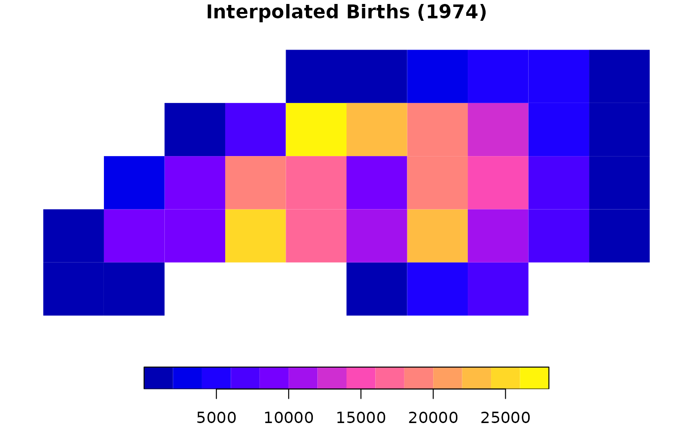
# Quick visualization
plot(result_ext["BIR74"], main = "Interpolated Births (1974)", border = NA)


# -------------------------------------------------------------------
# Example 4: Arrow ecosystem
# -------------------------------------------------------------------
# Export as geoarrow for zero-copy Parquet writing
geo_result <- sx_interpolate_aw(grid, nc, "tid", "sid", extensive = "BIR74", output = "geoarrow")
# }

Usage

Arguments

Value

Details

See also

Examples