2. Building analysis pipelines with targets

1 The targets package
1.1 What does the targets package do?
The {targets} package is a framework for building data processing, analysis and visualization pipelines in R. It helps you structure your code by splitting it onto logical chunks that follow each other in a logical order. {targets} also manages the intermediate results of each step, so you do not have to do it manually. It also minimizes the time it takes to update the results if any step changes, be it some change in the source data, or in the code. {targets} knows which steps are up-to-date, and which are not, and only runs the steps that are outdated.
Consider the following minimal example:
library(targets)

list(
  # 1. Load the mtcars dataset.
  tar_target(
    name = mtcars_data,
    command = data(mtcars)
  ),

  # 2. Compute the mean of the mpg column.
  tar_target(
    name = mpg_mean,
    command = mean(mtcars_data$mpg)
  ),

  # 3. Create a histogram plot of mpg using base R.
  tar_target(
    name = hist_mpg,
    packages = c("ggplot2"),
    command = {
      ggplot(mtcars_data, aes(x = mpg)) +
        geom_histogram(binwidth = 1) +
        labs(title = "Histogram of MPG", x = "Miles Per Gallon", y = "Count")
    }
  )
)
This script has three steps. It loads the data, computes a simple statistic, and creates a plot. To run this pipeline with targets you would need to save this script to the _targets.R file in the root of the project directory and run targets::tar_make() in R console.
Reveal code to try the toy targets example above in R console interactively
To quickly run the pipeline above in R console without setting up targets properly and creating an R script file, you can use the code below, that can be pasted in to the R console (and it will make the pipeline run in a temporary directory):
library(targets)
tar_dir({
  tar_script({
    library(targets)
    list(
      # Load the mtcars dataset.
      tar_target(mtcars_data, mtcars),

      # Compute the mean of the mpg column.
      tar_target(mpg_mean, mean(mtcars_data$mpg)),

      # Create a histogram plot of mpg using base R.
      # The plot is saved as a PNG file and the filename is returned.
      tar_target(plot_mpg, {
        png("hist_mpg.png")  # Open a PNG device.
        hist(mtcars_data$mpg,
             breaks = "Sturges",
             main = "Histogram of MPG",
             xlab = "Miles Per Gallon",
             ylab = "Frequency",
             col = "lightblue")
        dev.off()  # Close the device.
        "hist_mpg.png"  # Return the filename as the target value.
      })
    )
  }, ask = FALSE)

  # Run all targets defined in the pipeline.
  tar_make()

})
You will get output similar to this:
▶ dispatched target mtcars_data
● completed target mtcars_data [0 seconds, 1.225 kilobytes]
▶ dispatched target plot_mpg
● completed target plot_mpg [0.011 seconds, 65 bytes]
▶ dispatched target mpg_mean
● completed target mpg_mean [0 seconds, 52 bytes]
▶ ended pipeline [0.059 seconds]
It would mean that all steps have been executed successfully.
Similarly, if you add tar_visnetwork() after tar_make(), you will get a visualization of the pipeline:
library(targets)
tar_dir({
  tar_script({
    library(targets)
    list(
      # Load the mtcars dataset.
      tar_target(mtcars_data, mtcars),

      # Compute the mean of the mpg column.
      tar_target(mpg_mean, mean(mtcars_data$mpg)),

      # Create a histogram plot of mpg using base R.
      # The plot is saved as a PNG file and the filename is returned.
      tar_target(plot_mpg, {
        png("hist_mpg.png")  # Open a PNG device.
        hist(mtcars_data$mpg,
             breaks = "Sturges",
             main = "Histogram of MPG",
             xlab = "Miles Per Gallon",
             ylab = "Frequency",
             col = "lightblue")
        dev.off()  # Close the device.
        "hist_mpg.png"  # Return the filename as the target value.
      })
    )
  }, ask = FALSE)

  # Run all targets defined in the pipeline.
  tar_make()
  tar_visnetwork()
})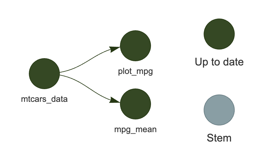
As you can see in Figure 1, {targets} knows that the summary statistic and the plot depend on the data. If you were to change the first step of the pipeline, then the next time you ask {targets} to update the pipeline, it would only run steps two and three. If, however, instead of changing the data, you changed the code for the plot (e.g. change the title), then the pipeline would only re-run step three. This way, you do not have to manually keep track of what might have changed in the data or the code, or, in more complex pipelines, in the intermediate data (such as cross-validation folds for machine learning models) - {targets} will figure it out for you.
2 Exercise
2.1 Goal
The goal of this exercise is to use the project folder that you have set up in the previous exercise with {renv} to create a simple analysis pipeline using {targets}.
If you have not successfully completed the previous exercise, you can start the current one by downloading the repository https://github.com/e-kotov/2025-mpidr-workflows-reference-01 and extracting it to your computer.
2.2 Instructions
2.3 Open the project folder in your editor
Open either your own project, or our reference project snapshot form the Note above.
If you open your own project, you should see in the R console:
- Project 'path/on/your/computer/to/your/project' loaded. [renv 1.1.1]If you open our reference project, you should see in the R console:
OK
- Installing renv  ... OK

- Project 'path/on/your/computer/2025-mpidr-workflows-reference-01' loaded. [renv 1.1.1]
- One or more packages recorded in the lockfile are not installed.
- Use `renv::status()` for more details.The reason you will see that the packages are not installed, is because the library of R packages is specific to an operating system and is considered as a disposable storage. By default, it is not pushed to GitHub. Therefore, when you copy such project from GitHub, you don’t have the packages, but you have all the files to restore the packages as required by the renv.lock file.
2.4 Restore (install) the R packages in the project
2.4.1 In your own project
In your own project, you need to run:
renv::status()This is to make sure that all the packages are installed in the project. If any packages are still missing, see the step below.
2.4.2 In our reference project
If you are working in our reference project from https://github.com/e-kotov/2025-mpidr-workflows-reference-01, you need to run:
renv::restore()After you confirm, you should see the package installation process.
Once the installation finishes, to make sure you have successfully installed all packages, run:
renv::status()You should get something like this:
No issues found -- the project is in a consistent state.2.5 Setup the {targets} pipeline
You could of course create a targets pipeline manually, but there is a handy R function to initialize a template for you:
targets::use_targets()Agree to that and {renv} will take over again to install a new package. Don’t forget to add it to the renv.lock file with renv::snapshot() later.
Once this is done, you should get a new file _targets.R in the root of your project folder.
2.6 Explore the sample pipeline
Before editing the _targets.R file, explore the pipeline that is already defined in the file.
First, run this to see the interactive graph of the pipeline (you will need to agree to install visNetwork package when you run this for the first time, run the command again if you still don’t see the visualisation in the viewer):
targets::tar_visnetwork()You will see that all steps are currently outdated.
Now you can runn all the steps in the pipeline:
targets::tar_make()Notice that you a new folder called _targets is created in the project folder. This is where the output of the pipeline will be stored as well as some metadata.
If you run targets::tar_visnetwork() again, you will find all steps are now up-to-date.
Now you can inspect in the R console the results of each step. You do not need to think where each output is saved, as all outputs are always stored in the _targets folder and are accessible by their name. For example:
tmp_object <- targets::tar_read(data)
print(tmp_object)
rm(tmp_object)
This will read the data object that is the output of the first step of the example pipeline and print it to the console. Finally, we also remove this object from the workspace to keep it clean.
You may also load the object data with its name directly into the workspace with:
targets::tar_load(data)ls()[1] "data"Now clean the workspace/environment:
rm(list = ls())To delete saved outputs of all or certain (see the documentation) steps, run:
targets::tar_destroy()To delete the saved results of steps that you might have deleted and will not use anymore, you could run:
targets::tar_prune()2.7 Adjust targets settings
Feel free to remove most of the comments in the example _targets.R file, especially the ones regarding the targets options. We recommend you do set the options as follows:
tar_option_set(
  format = "qs"
)
The qs/qs2 format is a faster and more space efficient alternative to rds format. You can read more about it in the qs2 documentation. This will be the format that targets uses to save the output of each step of the pipeline, unless you specify format = 'file', or set it to something else in the specicfic tar_target() step.
You might also notice that we suggest to remove the packages option from tar_option_set() that was originally there. This is because it is much safer to specify the packages you need in each tar_target() step individually. This might seem like a lot of work, but it it has many advatanges:
- Each step runs much faster, as unnecessary packages are not loaded.
- You can prevent potential package conflicts. In big projects with hundreds of packages, some packages may not work well when loaded simultaneously (which would happen if you specify the
packagesoption globally for all steps). - It is much easier to debug, as you can see which packages are loaded at each step.
For more targets options, you can see the documentation for tar_option_set().
2.8 Analysis step 1 - Get the data
See the code in Jonas’s repository at https://github.com/jschoeley/openscience25/tree/main/layer2-communal/example_2-1.
Let us try to implement the steps from his code in a targets pipeline. We will guide you through the first pipeline step together.
2.8.1 Wrap data download step into a function
We first need to implement the data download step found in https://github.com/jschoeley/openscience25/blob/main/layer2-communal/example_2-1/code/10-download_input_data_from_zenodo.R.
We will keep all functions that implement the steps in a separate folder called R. Create this folder manually and create a file called 10-download_input_data_from_zenodo.R in it. Copy the code from Jonas’s repository and save it in this new file, but convert it to a function that we could call from the targets pipeline. Compared to Jonas’s original code, this function needs to make sure that the folder for the file downloads exists and also return the paths to the downloaded data files. See the suggested function below:
# Download analysis input data from Zenodo
download_files_from_zenodo <- function(
  data_folder = "data"
) {
  # make sure the data folder exists
  if (!dir.exists(data_folder)) {
    dir.create(data_folder, recursive = TRUE)
  }

  # download the files
  download.file(
    url = 'https://zenodo.org/records/15033155/files/10-euro_education.csv?download=1',
    destfile = paste0(data_folder, "/10-euro_education.csv")
  )

  download.file(
    url = 'https://zenodo.org/records/15033155/files/10-euro_sectors.csv?download=1',
    destfile = paste0(data_folder, "/10-euro_sectors.csv")
  )

  download.file(
    url = 'https://zenodo.org/records/15033155/files/10-euro_geo_nuts2.rds?download=1',
    destfile = paste0(data_folder, "/10-euro_geo_nuts2.rds")
  )

  # find the downloaded files
  data_from_zenodo <- list.files("data", full.names = TRUE)

  # return the list of files
  return(data_from_zenodo)
}
Compare this to the original code from Jonas’s repository at https://github.com/jschoeley/openscience25/blob/main/layer2-communal/example_2-1/code/10-download_input_data_from_zenodo.R.
Now, to implement this first step into the pipeline, let us find the list of steps in the end of the _targets.R file, it’s the one where all the steps are listed, each starting with tar_target().
Remove all the example steps and insert your own:
list(
  # download files from zenodo
  tar_target(
    name = data_from_zenodo,
    command = download_files_from_zenodo(
      data_folder = "data"
    ),
    format = "file"
  )
)
Notice that we have added format = "file" to our first step. This means that targets should expect not a generic R object like a data.frame, list, or vector as on output of the download_files_from_zenodo() function, but a vector of files. This is useful for actions such as file downloads, as targets will be checking on it’s own if all expected files are actually downloaded.
The final step is to inform targets that we want to run the pipeline by executing the targets::tar_make().
2.8.2 Download files by executing the pipeline
Now you can run the pipeline by executing:
targets::tar_make()You should get something like this:
▶ dispatched target data_from_zenodo
trying URL 'https://zenodo.org/records/15033155/files/10-euro_education.csv?download=1'
Content type 'text/plain; charset=utf-8' length 11150 bytes (10 KB)
==================================================
downloaded 10 KB

trying URL 'https://zenodo.org/records/15033155/files/10-euro_sectors.csv?download=1'
Content type 'text/plain; charset=utf-8' length 20626 bytes (20 KB)
================================
downloaded 20 KB

trying URL 'https://zenodo.org/records/15033155/files/10-euro_geo_nuts2.rds?download=1'
Content type 'application/octet-stream' length 261344 bytes (255 KB)
=======
downloaded 255 KB

● completed target data_from_zenodo [0.894 seconds, 293.12 kilobytes]
▶ ended pipeline [0.94 seconds]
The pipeline downloaded the files from Zenodo and will save them into the data folder. You can now use the downloaded files in the next steps of the pipeline.
Make an interactive graph of the pipeline:
targets::tar_visnetwork()You should see a network similar to the one in Figure 2.
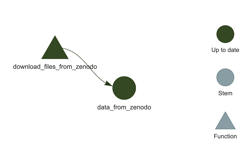
One thing to try, is to manually delete any one of the downloaded files and run the targets::tar_visnetwork() function. You will then see that one of the steps is outdated, as targets knows from the first run that it needs to keep track of files and it has noted the file signatures.
2.8.3 Add data folder to .gitignore
As the data is preserved at Zenodo, and as it is bad practice to store data in the git repository, we should add the data folder to the .gitignore file. You can do this by executing the following command in the R console:
usethis::use_git_ignore("data")This will create a new .gitignore file in the root of the project (in case it did not exist) and add the data folder there. Now git tools will not prompt you to commit the data folder and it will never be pushed to GitHub or other remote repository you are using.
2.9 Analysis step 2 - Create background map
Now let us add a new step that creates background map that will be re-used in all of the plots me can create following the code in Jonas’s repository. We will look at the code in https://github.com/jschoeley/openscience25/blob/main/layer2-communal/example_2-1/code/20-create_european_backgroundmap.R and adjust it to be a targets step executed by tar_target().
Because the code there uses _config.yaml to customize the plots, you will need to download it and put into your project, e.g. into config folder.
We will also break down the code into steps, as it makes sense to isolate the code for downloading the data from Natural Earth into a separate function.
2.9.0.1 Step 2.1 Download Natural Earth data
Look at the corresponding lines in Jonas’s code:
# Download Eurasian geodata ---------------------------------------
eura_sf <-
  # download geospatial data for European, Asian and African countries
  ne_countries(continent = c('europe', 'asia', 'africa'),
               returnclass = 'sf', scale = 10) %>%
  # project to crs suitable for Europe
  st_transform(crs = config$crs) %>%
  # merge into single polygon
  st_union(by_feature = FALSE) %>%
  # crop to Europe
  st_crop(xmin = config$eurocrop$xmin,
          xmax = config$eurocrop$xmax,
          ymin = config$eurocrop$ymin,
          ymax = config$eurocrop$ymax)
We will rewrite it as a following function:
# Download Eurasian geodata ---------------------------------------
download_ne_data <- function(
  crs, xmin, xmax, ymin, ymax
) {
  eura_sf <-
    # download geospatial data for European, Asian and African countries
    rnaturalearth::ne_countries(
      continent = c('europe', 'asia', 'africa'),
      returnclass = 'sf',
      scale = 10
    ) |>
    # project to crs suitable for Europe
    sf::st_transform(crs = crs) |>
    # merge into single polygon
    sf::st_union(by_feature = FALSE) |>
    # crop to Europe
    sf::st_crop(xmin = xmin, xmax = xmax, ymin = ymin, ymax = ymax)

  return(eura_sf)
}
As you can see, we got rid of the references to yaml file, which is one of the ways to approach it. Any preferences previously set in yaml file are now set in the function parameters.
We also prefixed each function call with a package name. We do this to be more aware of which packages we use in each function to minimize the potential for conflicts.
In the list of targets steps we will add the call as follows:
tar_target(
  name = eura_sf,
  packages = c("rnaturalearth", "sf"),
  command = download_ne_data(
    crs = 3035,
    xmin = 25.0e+5,
    xmax = 75.0e+5,
    ymin = 13.5e+5,
    ymax = 54.5e+5
  )
)
Note that:
- We specified the
packagesargument for an individual target step. - We did not specify the
format = "file", so by default it will beqs2format, as specified above intar_option_set().
As you might have noticed, we set the name of the targets step as eura_sf, and we also return an object called eura_sf from the download_ne_data() function. These names do NOT have to match, as in larger projects functions may be reused multiple times and they may have more generic uses and therefore return different output to different targets based on their input parameters. In this case, we are just naming the objects in the same way for convenience.
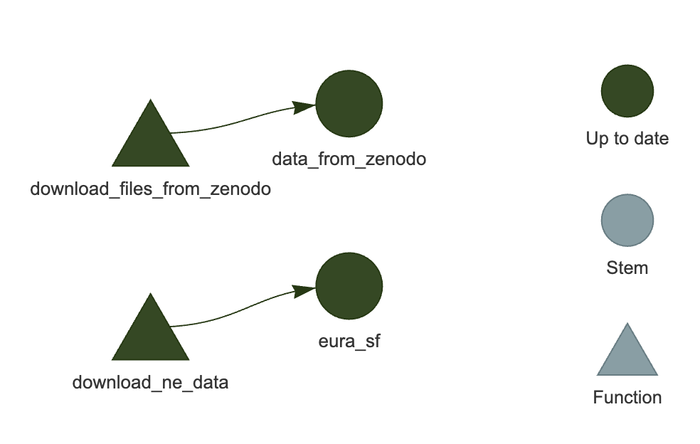
Test the targets pipeline by running it and making an interactive graph:
targets::tar_make()
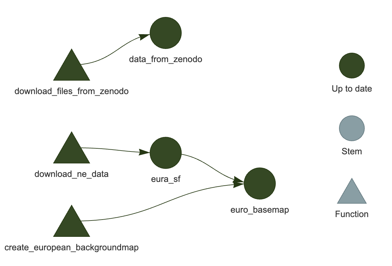
targets::tar_visnetwork()You should see a network similar to the one in Figure 3.
2.10 Step 2.2 Wrap background map creation step into a function
Create a file 20-create_european_backgroundmap.R in R subfolder of your project.
Look at the first few lines in Jonas’s code, just after the library() calls (which we will look at later).
Original lines:
# input and output paths
paths <- list()
paths$input <- list(
  config = './code/_config.yaml'

)
paths$output <- list(
  euro_basemap.rds = './data/20-euro_basemap.rds'
)

# global configuration
config <- read_yaml(paths$input$config)
We do not nede to use any of these lines anymore. Previously we had to specify where to save the base map in paths$output. With targets, we do not need to manually keep track where we save intermediate results and wether or not they are up to date. Instead of saving the file at the path specified in paths$output, we will just return an R object from the function called by a particular targets step and it will be stored automatically for us in _targets/objects folder. We do not need the _config.yaml here anymore, as it did not contain any variables that would affect the basemap creation.
We only need the lines that create a ggplot2 plot object with the basemap:
# Draw a basemap of Europe ----------------------------------------
euro_basemap <-
  ggplot(eura_sf) +
  geom_sf(
    aes(geometry = geometry),
    color = NA, fill = 'grey90'
  ) +
  coord_sf(expand = FALSE, datum = NA) +
  theme_void()
And we rewrite these as a function:
# Draw a basemap of Europe ----------------------------------------
create_european_backgroundmap <- function(
  eura_sf
) {
  # eura_sf <- targets::tar_read(eura_sf) # for debug

  euro_basemap <-
    ggplot2::ggplot(eura_sf) +
    ggplot2::geom_sf(
      aes(geometry = geometry),
      color = NA,
      fill = 'grey90'
    ) +
    ggplot2::coord_sf(expand = FALSE, datum = NA) +
    ggplot2::theme_void()

  return(euro_basemap)
}
Notice that we pass eura_sf object that we created with targets step that executed download_ne_data() and we return the ggplot2 object euro_basemap that should be reused in the next steps for creating the maps.
We also added explicit ggplot2:: prefixes to relevant functions. This is optional, as we will specify that we need ggplot2 package for this function in the targets pipeline, but this also helps to debug the function quickly.
To run the code in this function manually, you can use the commented out line eura_sf <- targets::tar_read(eura_sf) to quickly load the eura_sf object (assuming you have previously ran the targets pipeline and it is saved in the targets/ojects storage).
Now let us add a targets step to the pipeline:
tar_target(
  name = euro_basemap,
  packages = c("ggplot2"),
  command = create_european_backgroundmap(
    eura_sf = eura_sf
  )
)
Test the targets pipeline by running it and making an interactive graph:
targets::tar_make()
targets::tar_visnetwork()
You should see a network similar to the one in Figure 4.
Now if you run targets::tar_read(euro_basemap), you should get a plot of the basemap (see Figure 5):

targets::tar_read(euro_basemap)
2.11 Next steps
Now you it is up to you to adapt the code from one of the R scripts that create maps (30-plot_figure_1.R, 31-plot_figure_2.R, 32-plot_figure_3.R) in Jonas’s repository at https://github.com/jschoeley/openscience25/tree/main/layer2-communal/example_2-1/code. in the same way we did above. We would suggest that because these plots are final output images, instead of returning ggplot2 objects from the plot making functions, you save the plots to files and return the path to the file, like we did with the step that downloaded the data from Zenodo.